Dynamic Inventory | Ender Sari

Dynamic Inventory and Production Management

My primary objective was to enhance inventory management and production planning processes to prevent stockouts, ensure timely deliveries, and better align production with fluctuating demand patterns. Also, I wanted to develop a more flexible and responsive system that leverages data-driven decision-making to optimize operations.

Methodology:

Dynamic Target Weekly Cover Value (TWCV): I led the development of an innovative algorithm that dynamically adjusts the TWCV for each product based on demand volatility, with a variable range of 2 to 5 weeks.
Advanced Analytics for Capacity Planning: Advanced analytics were employed to accurately calculate monthly production capacities and forecast demands. The Capacity Utilization (CU) metric was introduced as a strategic tool to guide production decisions based on the ratio of forecasted demand to production capacity.
Responsive Inventory Adjustments: A system was implemented allowing TWCV to dynamically change throughout the year, enabling proactive inventory adjustments in response to anticipated demand fluctuations and constraints from SKU-specific mold capacities.

The integration of these strategies shifted the tire manufacturer towards a more data-driven decision-making framework. This approach improved production scheduling and reduced inventory levels for most products, thereby lowering holding costs and enhancing operational efficiency. However, it also highlighted increased inventory levels in some products, indicating areas for further optimization.

You can access the sample Python notebook code.

Button

In my sample calculation, for each product I used the beginning inventory levels, and the monthly demand forecasts and production capacity values. The figure at the bottom summarizes how the calculated capacity utilization values are related to production decisions. The threshold values 0.25, 0.50, 0.75 arise due to the simplified month-week conversion: If the CU is less than 0.25, then at most one-week of production would be sufficient to meet the forecasted monthly demand. I added a buffer of one week to obtain the assigned TWCV values for each group in the table.

algorithm

TWCV for the t months in the decision horizon is calculated with the algorithm at the bottom. The weight W is used for smoothing the potential fluctuation of TWCV between consecutive months. To achieve smoothing, the algorithm considers the CU values in four months, and takes a weighted average of the maximum of CUt and CUt+1, and the maximum of CUt+2 and CUt+3. By doing so, I allowed the monthly TWCV to change by a maximum of 1 week consecutive months. In the absence of such smoothing it would be difficult to ramp up the inventory to targeted values.

result

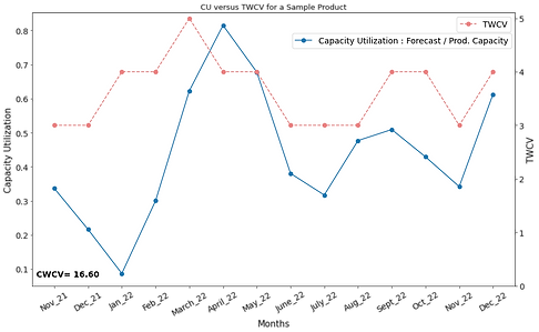
Next, I illustrate the capacity utilization (forecast / production capacity) and TWCV calculations for the 14-month horizon for our sample product. The left axis and the blue line show the capacity utilization values; whereas, red dashed line, and the right axis show the targeted weekly cover values. As for the weight value W is chosen as 0.60. We observe the CU values to decrease until January, and then increase significantly until April, after which they decrease again. To prepare for this increase in capacity utilization, the algorithm increases the TWCV from November until March, and decreases them afterwards till August.

This process will be used to determine production quantities. At the beginning of each week, for each product that is sold in the OE channel, the current and target weekly cover values will be compared. Products for which CWCV < TWCV will be flagged for production. Even though the company gives priority to a speficic channel products, there may not be sufficient overall production capacity to produce all of the required products in the coming weeks. Hence, each product will be assigned a production priority score that is based on the difference between TWCV and CWCV, customer priority and the gross profit margin of the product. Also, I compare the inventory levels that would be realized under my suggestion with the realized values as of November 2021. Figure below compares these for 11 popular products from passenger tire category. I observe that for most products, my procedure would have resulted in lower amounts of inventory while for some products the opposite is the case. Overall, I reduced the beginning inventory levels by 20 percent.

inspiration

Inspired by the dynamic shifts in inventory management, I have crafted innovative strategies that tackle emerging challenges and seize new opportunities in this ever-evolving field. If you're curious about the underlying literature that informs these strategies, please keep reading for a deeper dive into influential research.

Quantity-based policies assume demand distribution to be stationary, that is not to change over time (Nahmias and Olsen, 2015; Silver et al., 1998). Stationary demand distribution assumption is not a suitable one for most real-life cases, especially for products that exhibit strongly seasonal demand or demand with spikes due to bulk ordering, as is the case for the company we consider. Demand may change over time based on the product life-cycle stage, marketing activities, competitor activities or cannibalization due to the introduction of a substitute product of the firm.

A practical alternative to quantity-based policies that can handle nonstationary demand is the cover-based policies (Hoppe, 2006). These are also known as Inventory days of supply. In a cover-based policy, the target inventory level is expressed not as a quantity but as the number of time units (days, weeks or months) for which the inventory level shall cover the forecasted demand (King and King, 2017) in the subsequent time periods. Cover based policies are especially popular in business practice due to their ability to handle non-steady demand, as well as their ease of application in ERP systems and ease of explanation.

References:

King, P. L. and King, J. S. (2017). Value stream mapping for the process industries:Creating a roadmap for lean transformation. CRC Press.
Hoppe, M. (2006). Inventory optimization with SAP, volume 477. Sap PressGaithersburg, MD.
Nahmias, S. and Olsen, T. L. (2015). Production and operations analysis. WavelandPress.